Table of Contents
Intro
In fantasy football, volume will always be king. That being said, not all volume is necessarily equal. A running back who gets five carries inside the five yard line will be far more valuable than a running back who gets five carries 80 yards from the end zone because of the likelihood of the first player scoring a touchdown. Touchdowns (and other big plays) have an outsized significance in fantasy, and advanced play-by-play data can help us identify instances where players are overachieving at an unsustainable rate.
In early August of this year, Ben introduced a model that will estimate yards after the catch based on air yards, down & distance, yard line, and a number of other factors. The model provides the probability that a player will advance to any particular yard line, given that they make the catch. Upon seeing this, I was immediately reminded of an article I had seen some time ago by Mike Clay, which was aimed at estimating the opportunity a player had to score a touchdown based on where they received the ball. Since nflfastR already has a completion probability model, it would be relatively simple to combine these models together to calculate the outcome of any single result for a given pass play. I shared some initial thoughts/visuals on twitter for this idea, and I thought it would be great if others had some code to play around with this as well.
Something important to remember about this concept is that it merely calculates expected fantasy points for the average receiver. Receivers who are especially skilled at gaining yards after the catch or who catch more passes than expected will typically over perform their mean expectation on this metric. I’ll also add to the latter point: we can say with some degree of confidence that, all else being equal, the quarterback is most likely more responsible for completing a pass than the receiver. This means that for the purposes of the expected fantasy points we’ll be calculating below, we should take the quality of quarterback into account.
All of this code will be written for PPR scoring, but it would not be difficult to adjust any of this for standard scoring, half-point PPR, or even Scott Fish Bowl scoring (although you would need some kind of roster table to look up positions). I will also add that this will not take fumbles, two-point conversions, or rushing plays into account.
The YAC Distribution Function
As of this writing, nflfastR does not have a built-in function that provides the full distribution of outcomes for YAC on each play. While that may be available at some point in the future, the easiest solution right now is to make our own adjustments to the add_xyac function so that we can get the raw xYAC model output. The intended purpose of add_xyac is to add five fields (xyac_epa, xyac_success, xyac_fd, xyac_mean_yardage, and xyac_median_yardage) to the play-by-play data frame. We’re going to break the function up into blocks, remove 12 rows that basically serve to summarize the model output, and reassemble it so that the function will return a row for each possible yardage outcome. While we won’t actually be need nflfastR library for this, we will be sourcing the file that has the xyac functions and also the file that makes some mutations.
library(tidyverse)

source('https://github.com/mrcaseb/nflfastR/raw/master/R/helper_add_xyac.R')
source('https://github.com/mrcaseb/nflfastR/raw/master/R/helper_add_nflscrapr_mutations.R')

# duplicate the add_xyac() function that we sourced above
add_xyac_dist <- add_xyac

# separate each block of code in the add_xyac_dist() function into blocks
add_xyac_blocks <- body(add_xyac_dist) %>% as.list

# we want to remove lines 51 to 62 from the 5th item in the list
add_xyac_blocks[[5]] <- add_xyac_blocks[[5]] %>%
  format %>%
  .[-(51:62)] %>%
  paste(collapse = '\n') %>%
  str2lang

# replace the body of add_xyac_dist() with our new edited function
body(add_xyac_dist) <- add_xyac_blocks %>% as.call
The Data
Now that we’ve got our function squared away, we can focus on assembling the data. We’ll pull in the 2019 data set and keep only regular season pass plays from scrimmage where a player was actually targeted. The table we ultimately create will summarize expected stats and actual stats for each player last season. This can obviously be summarized at the game level as well.
pbp_df <- readRDS(url('https://raw.githubusercontent.com/guga31bb/nflfastR-data/master/data/play_by_play_2019.rds'))

avg_exp_fp_df <- pbp_df %>%
  filter(pass_attempt==1 & season_type=='REG' & two_point_attempt==0 & !is.na(receiver_id)) %>%
  add_xyac_dist %>%
  select(season = season.x, game_id, play_id, posteam = posteam.x, receiver, yardline_100 = yardline_100.x, air_yards = air_yards.x, actual_yards_gained = yards_gained, complete_pass, cp, yac_prob = prob, gain) %>%
  mutate(
    gain = ifelse(yardline_100==air_yards, yardline_100, gain),
    yac_prob = ifelse(yardline_100==air_yards, 1, yac_prob),
    PPR_points = 1 + gain/10 + ifelse(gain == yardline_100, 6, 0),
    catch_run_prob = cp * yac_prob,
    exp_PPR_points = PPR_points * catch_run_prob,
    exp_yards = gain * catch_run_prob,
    actual_outcome = ifelse(actual_yards_gained==gain & complete_pass==1, 1, 0),
    actual_PPR_points = ifelse(actual_outcome==1, PPR_points, 0),
    target = 0,
    game_played = 0
  )  %>%
  group_by(game_id, receiver) %>%
  mutate(game_played = ifelse(row_number()==1,1,0)) %>%
  ungroup %>%
  group_by(game_id, play_id, receiver) %>%
  mutate(target = ifelse(row_number()==1,1,0)) %>%
  ungroup %>%
  group_by(posteam, receiver) %>%
  summarize(
    games = sum(game_played, na.rm = T),
    targets = sum(target, na.rm = T),
    catches = sum(actual_outcome, na.rm = T),
    yards = sum(ifelse(actual_outcome==1, gain, 0), na.rm = T),
    td = sum(ifelse(gain==yardline_100, actual_outcome, 0), na.rm = T),
    PPR_pts = sum(actual_PPR_points, na.rm = T),
    exp_catches = sum(ifelse(target==1, cp, NA), na.rm = T),
    exp_yards = sum(exp_yards, na.rm = T),
    exp_td = sum(ifelse(gain==yardline_100, catch_run_prob, 0), na.rm = T),
    exp_PPR_pts = sum(exp_PPR_points, na.rm = T)
  ) %>%
  ungroup
Let’s make a table using the gt package to show the top 25 players in expected fantasy points last season. It looks like OBJ under performed pretty severely, while Cooper Kupp scored about four and a half more TDs than expected!
library(gt)

# make the table
avg_exp_fp_df %>%
  arrange(-exp_PPR_pts) %>%
  dplyr::slice(1:25) %>%
  mutate(Rank = paste0('#',row_number())) %>%
  gt() %>%
  tab_header(title = 'Expected Receiving PPR Fantasy Points, 2019') %>%
  cols_move_to_start(columns = vars(Rank)) %>%
  cols_label(
    games = 'GP',
    receiver = '',
    posteam = '',
    targets = 'Targ',
    catches = 'Rec',
    yards = 'Yds',
    td = 'TD',
    PPR_pts = 'FP',
    exp_catches = 'Rec',
    exp_yards = 'Yds',
    exp_td = 'TD',
    exp_PPR_pts = 'FP'
  ) %>%
  fmt_number(columns = vars(exp_td, PPR_pts, exp_PPR_pts), decimals = 1) %>%
  fmt_number(columns = vars(yards, exp_yards, exp_catches), decimals = 0, sep_mark = ',') %>%
  tab_style(style = cell_text(size = 'x-large'), locations = cells_title(groups = 'title')) %>%
  tab_style(style = cell_text(align = 'center', size = 'medium'), locations = cells_body()) %>%
  tab_style(style = cell_text(align = 'left'), locations = cells_body(vars(receiver))) %>%
  tab_spanner(label = 'Actual', columns = vars(catches, yards, td, PPR_pts)) %>%
  tab_spanner(label = 'Expected', columns = vars(exp_catches, exp_yards, exp_td, exp_PPR_pts)) %>%
  tab_source_note(source_note = '') %>%
  data_color(
    columns = vars(PPR_pts, exp_PPR_pts),
    colors = scales::col_numeric(palette = c('grey97', 'darkorange1'), domain = c(180,380)),
    autocolor_text = FALSE
  ) %>%
  text_transform(
    locations = cells_body(vars(posteam)),
    fn = function(x) web_image(url = paste0('https://a.espncdn.com/i/teamlogos/nfl/500/',x,'.png'))
  ) %>%
  cols_width(vars(posteam) ~ px(45)) %>%
  tab_options(
    table.font.color = 'darkblue',
    data_row.padding = '2px',
    row_group.padding = '3px',
    column_labels.border.bottom.color = 'darkblue',
    column_labels.border.bottom.width = 1.4,
    table_body.border.top.color = 'darkblue',
    row_group.border.top.width = 1.5,
    row_group.border.top.color = '#999999',
    table_body.border.bottom.width = 0.7,
    table_body.border.bottom.color = '#999999',
    row_group.border.bottom.width = 1,
    row_group.border.bottom.color = 'darkblue',
    table.border.top.color = 'transparent',
    table.background.color = '#F2F2F2',
    table.border.bottom.color = 'transparent',
    row.striping.background_color = '#FFFFFF',
    row.striping.include_table_body = TRUE
)| Expected Receiving PPR Fantasy Points, 2019 | ||||||||||||
|---|---|---|---|---|---|---|---|---|---|---|---|---|
| Rank | GP | Targ | Actual | Expected | ||||||||
| Rec | Yds | TD | FP | Rec | Yds | TD | FP | |||||
| #1 |  |
M.Thomas | 16 | 185 | 149 | 1,725 | 9 | 375.5 | 128 | 1,480 | 6.8 | 317.2 |
| #2 |  |
J.Jones | 15 | 157 | 99 | 1,394 | 6 | 274.4 | 98 | 1,444 | 6.7 | 282.1 |
| #3 |  |
A.Robinson | 16 | 154 | 98 | 1,147 | 7 | 254.7 | 95 | 1,311 | 7.2 | 269.4 |
| #4 |  |
D.Hopkins | 15 | 150 | 104 | 1,165 | 7 | 262.5 | 98 | 1,251 | 7.4 | 267.3 |
| #5 |  |
J.Edelman | 16 | 153 | 99 | 1,117 | 6 | 246.7 | 100 | 1,230 | 6.8 | 263.7 |
| #6 |  |
K.Allen | 16 | 149 | 104 | 1,199 | 6 | 259.9 | 93 | 1,192 | 6.9 | 253.3 |
| #7 |  |
T.Boyd | 16 | 148 | 90 | 1,046 | 5 | 224.6 | 96 | 1,193 | 4.5 | 241.8 |
| #8 |  |
T.Kelce | 16 | 136 | 96 | 1,248 | 5 | 250.8 | 88 | 1,066 | 6.8 | 235.7 |
| #9 |  |
O.Beckham | 16 | 133 | 73 | 946 | 3 | 185.6 | 80 | 1,147 | 6.7 | 235.1 |
| #10 |  |
Z.Ertz | 15 | 135 | 88 | 916 | 6 | 215.6 | 88 | 1,063 | 6.7 | 234.4 |
| #11 |  |
D.Parker | 16 | 128 | 72 | 1,202 | 9 | 246.2 | 75 | 1,169 | 6.9 | 232.9 |
| #12 | |
J.Landry | 16 | 138 | 83 | 1,180 | 6 | 237.0 | 85 | 1,093 | 6.3 | 232.5 |
| #13 |  |
D.Moore | 15 | 135 | 87 | 1,175 | 4 | 228.5 | 84 | 1,120 | 5.7 | 230.5 |
| #14 |  |
M.Evans | 13 | 118 | 67 | 1,157 | 8 | 230.7 | 65 | 1,076 | 9.5 | 229.7 |
| #15 |  |
K.Golladay | 16 | 116 | 65 | 1,190 | 11 | 250.0 | 65 | 1,060 | 9.6 | 229.1 |
| #16 |  |
R.Woods | 15 | 139 | 90 | 1,134 | 2 | 215.4 | 92 | 1,118 | 3.8 | 227.1 |
| #17 |  |
D.Adams | 12 | 127 | 83 | 997 | 5 | 212.7 | 82 | 997 | 7.4 | 225.9 |
| #18 |  |
C.Sutton | 16 | 124 | 72 | 1,112 | 6 | 219.2 | 73 | 1,020 | 7.7 | 221.0 |
| #19 | |
C.Kupp | 16 | 134 | 94 | 1,161 | 10 | 270.1 | 89 | 977 | 5.6 | 220.1 |
| #20 | |
C.Godwin | 14 | 121 | 86 | 1,333 | 9 | 273.3 | 76 | 1,024 | 6.3 | 216.7 |
| #21 |  |
A.Cooper | 16 | 119 | 79 | 1,189 | 8 | 245.9 | 74 | 1,109 | 5.2 | 215.7 |
| #22 | |
C.McCaffrey | 16 | 142 | 116 | 1,005 | 4 | 240.5 | 112 | 825 | 3.1 | 213.8 |
| #23 |  |
D.Chark Jr. | 15 | 118 | 73 | 1,008 | 8 | 221.8 | 72 | 987 | 6.8 | 211.0 |
| #24 |  |
T.Lockett | 16 | 110 | 82 | 1,057 | 8 | 235.7 | 65 | 906 | 7.6 | 201.1 |
| #25 |  |
J.Brown | 15 | 115 | 72 | 1,060 | 6 | 214.0 | 65 | 1,039 | 4.9 | 198.8 |
The Distribution
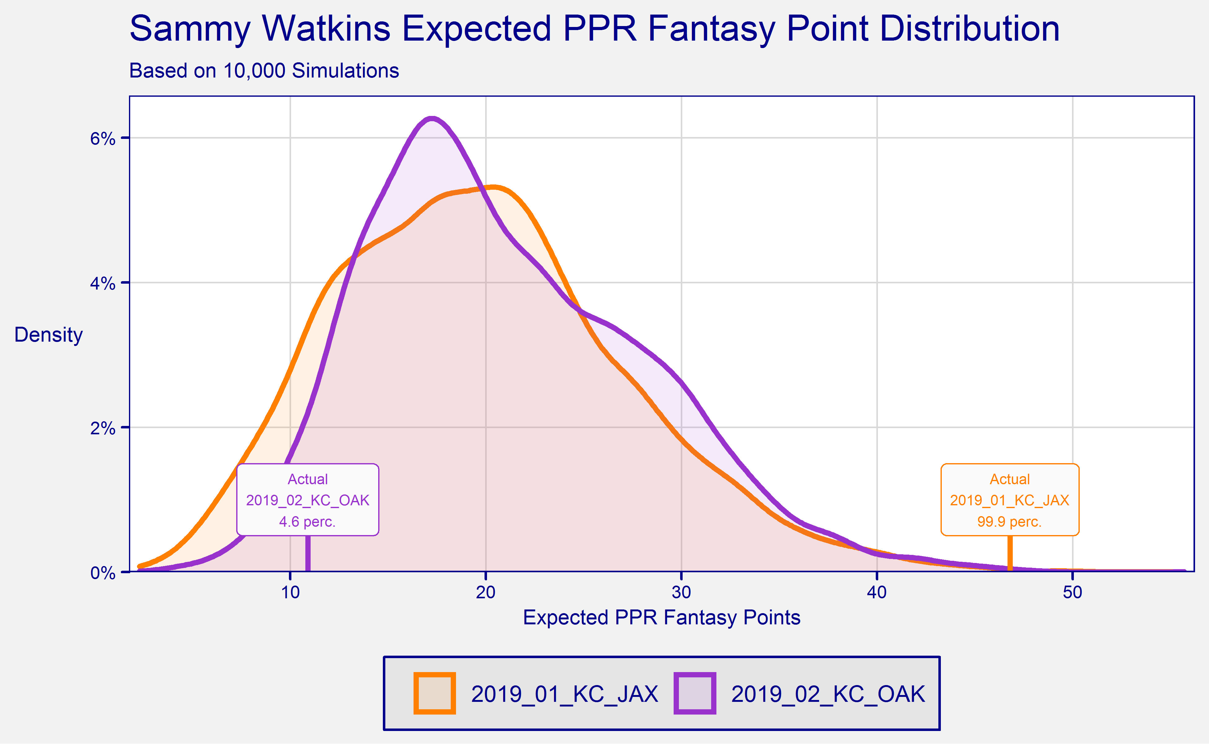
Estimating the mean is informative, but doesn’t give us much depth. A great thing about these models is they make it easy to estimate the distribution of outcomes for expected fantasy points. For this example, let’s take a look at Sammy Watkins Week 1 explosion and subsequent Week 2 letdown from last season.
fant_pt_dist_df <- pbp_df %>%
  filter(pass_attempt==1 & season_type=='REG' & two_point_attempt==0 & !is.na(receiver_id) & receiver == 'S.Watkins' & week <= 2) %>%
  add_xyac_dist %>%
  select(season = season.x, game_id, play_id, posteam = posteam.x, receiver, yardline_100 = yardline_100.x, air_yards = air_yards.x, actual_yards_gained = yards_gained, complete_pass, cp, yac_prob = prob, gain) %>%
  mutate(
    gain = ifelse(yardline_100==air_yards, yardline_100, gain),
    yac_prob = ifelse(yardline_100==air_yards, 1, yac_prob),
    PPR_points = 1 + gain/10 + ifelse(gain == yardline_100, 6, 0),
    catch_run_prob = cp * yac_prob,
    exp_PPR_points = PPR_points * catch_run_prob,
    actual_outcome = ifelse(actual_yards_gained==gain & complete_pass==1, 1, 0),
    actual_PPR_points = ifelse(actual_outcome==1, PPR_points, 0),
    target = 0,
    game_played = 0
  )

incomplete_df <- fant_pt_dist_df %>%
  mutate(
    gain = 0,
    PPR_points = 0,
    yac_prob = 0,
    exp_PPR_points = 0,
    complete_pass = 0,
    catch_run_prob = 1 - cp,
    actual_outcome = NA,
    actual_PPR_points = NA,
    target = 1
  ) %>%
  distinct %>%
  group_by(game_id, receiver) %>%
  mutate(game_played = ifelse(row_number()==1,1,0)) %>%
  ungroup
Now we can take the outcomes above and simulate each play 10,000 times and summarize them at the player level. This will take a couple of minutes in this case, but may take a bit more time depending on the number of plays you’re trying to simulate outcomes for.
# make a data frame to loop around
sampling_df <- rbind(incomplete_df, fant_pt_dist_df) %>%
  select(season, game_id, play_id, posteam, receiver, catch_run_prob, PPR_points) %>%
  group_by(game_id, play_id)

# do sim
sim_df <- do.call(rbind, lapply(1:10000, function(x) {
  sampling_df %>%
    mutate(sim_res = sample(PPR_points, 1, prob = catch_run_prob)) %>%
    select(season, game_id, play_id, posteam, receiver, sim_res) %>%
    distinct %>%
    group_by(game_id, posteam, receiver) %>%
    summarize(sim_tot = sum(sim_res, na.rm = T), .groups = 'drop') %>%
    return
}))

sim_df <- sim_df %>% mutate(sim = 1)

# calculate how many points were actually scored
actual_df <- fant_pt_dist_df %>%
  group_by(game_id, posteam, receiver) %>%
  summarize(sim_tot = sum(actual_PPR_points, na.rm = T), .groups = 'drop') %>%
  mutate(sim = 0)

# figure out what percentile the actual values fall in
percentile_df <- rbind(sim_df, actual_df) %>%
  group_by(game_id, posteam, receiver) %>%
  mutate(perc = percent_rank(sim_tot)) %>%
  filter(sim == 0)
Watkins converted his 11 targets into 9 catches for 198 yards and three scores in Week 1, good for 46.8 PPR fantasy points which is in the 99th percentile of the outcomes that we simulated. Despite being targeted 13 times in Week 2, Watkins finished with a mere 10.9 PPR fantasy points. This outcome fell in the 4th percentile.
library(scales)


ggplot(data = sim_df, aes(x = sim_tot, group = game_id, color = game_id, fill = game_id)) +
  geom_density(alpha = 0.1, size = 1) +
  geom_spoke(data = percentile_df, aes(angle = pi/2, radius = 0.01, y = 0), size = 1, show.legend = F)  +
  geom_label(data = percentile_df, aes(y = 0.01, label = paste0('Actual\n',game_id,'\n',number(round(perc*100,2),accuracy = 0.1), ' perc.')), size = 2, fill = 'grey98', show.legend = F)  +
  scale_x_continuous(expand = expansion(mult = c(0.01, 0.01))) +
  scale_y_continuous(labels = percent_format(accuracy = 1), expand = expansion(mult = c(0, 0.05))) +
  scale_color_manual(values = c('#ff7f00','#9932cc')) +
  scale_fill_manual(values = c('#ff7f00','#9932cc')) +
  labs(title = 'Sammy Watkins Expected PPR Fantasy Point Distribution',
       subtitle = 'Based on 10,000 Simulations',
       y = 'Density',
       x = 'Expected PPR Fantasy Points',
       color = NULL,
       fill = NULL) +
  theme(
    line = element_line(lineend = 'round', color='darkblue'),
    text = element_text(color='darkblue'),
    plot.background = element_rect(fill = 'grey95', color = 'transparent'),
    panel.border = element_rect(color = 'darkblue', fill = NA),
    panel.background = element_rect(fill = 'white', color = 'transparent'),
    axis.ticks = element_line(color = 'darkblue', size = 0.5),
    axis.ticks.length = unit(2.75, 'pt'),
    axis.title = element_text(size = 8),
    axis.text = element_text(size = 7, color = 'darkblue'),
    plot.title = element_text(size = 14),
    plot.subtitle = element_text(size = 8),
    plot.caption = element_text(size = 5),
    legend.background = element_rect(fill = 'grey90', color = 'darkblue'),
    legend.key = element_blank(),
    panel.grid.minor = element_blank(),
    panel.grid.major = element_line(color='grey85', size = 0.3),
    axis.title.y = element_text(angle = 0, vjust = 0.5),
    legend.position = 'bottom'
) 
Comparing Watkins’ first two weeks, one could reasonably assume that he would eventually steady out in the high teens or low 20s and wind up as a top three option by the end of the season. Unfortunately, Watkins was unable to retain his target share (volume is still king!) and later missed essentially three games due to injury.
This example captures the strengths and weakness of this process pretty well. On one hand, we’ve identified that Kansas City’s offense is capable of serving up a juicy fantasy game (shocker). We also were able to set more realistic expectations for Sammy Watkins moving forward by dismissing some outlier performances. On the other hand, we still can’t assume any single game is incredibly predictive week-to-week, as Watkins relinquished his alpha role shortly after these performances. A lot of a receiver’s volume will ultimately depend on the game script and health of his peers.
Next Steps
There is plenty of room to explore this approach further, especially when it comes to making this metric more predictive. One thought I’ve had is to incorporate a prior for the CPOE of starting QB and YAC over expected for the receiving player. The YAC & CP models also might look different if positions were taken into account. They are not included in the model as of this writing due to concerns over data availability. I would also be interested in seeing how this might look for QBs, although fantasy points from rushing plays would be excluded. In theory, one could create a rushing play model in the same way as the xYAC model.
Big thanks to Ben & Sebastian for creating and maintaining the models used here. This would have been impossible without them!